Contents
目标
这个作业的目标是,训练出一个网络,给它32×32图片作为输入,它能判断出这个图片代表什么交通标识。
这个网络基于 LeNet, 所以本文会先讲述 DNN 和 CNN 的一些基础知识,再讨论作业的代码实现和训练过程。
DNN – Deep Neural Networks
单层网络 f=WX+b 只能进行线性转换,难以进行复杂的判断。通过堆积多层网络,添加非线性的元素(如activation layer),使得网络可以处理更负责的情况。
Activation
Activation Layer 可以提供“非线性”,在一定情况下会被“触发”,而其余情况则不会被“触发”,模拟神经细胞的行为。
常见的 Activation Functions 有 Sigmoid, tanh, ReLU, Leaky ReLU, Maxout, ELU. 实际中,通常会使用 ReLU.

Sigmoid 处处可导,可以把输出范围控制在[0,1]区间。不过,它的一个大问题是会kill gradient。假设输入是10,那么做bp的时候,就会得到接近于无限大的数。如果输入是-10,则可能得到负无限的数,这样的bp得到的结果没有意义。
另外一个问题是,它的输出不是 zero-centered 的 (中心在0.5)。

tanh可以做到 zero-centered,不够还是会 kill gradient.

ReLU 比较粗暴简单,大于0的输入原封不动输出,小于0的输出为0,节省计算资源。不过它的输出也不是 zero-centered 的,且对于输入小于0的部分,在bp时gradient永远得不到更新。

Leaky ReLU 在小于0的部分输出一个按比例缩小的数,使得gradient在bp时仍然可以传递。

ELU 也解决了输入小于0得不到更新的问题,不过它需要用到 exp(),计算开销大。

Maxout 类似一种通用的leaky ReLU, 用两套 weights 来对输入进行运算,谁大谁出。问题也很明显,weights 的数量翻倍了,多出了要训练的东西。

Regularization/Dropout
训练一个网络,我们很容易遇到 overfitting 的问题。(训练错误率越来越低,但测试错误率越来越高)
缓解这个问题,可以采取一些 Regularization 的手段,防止 weights 过调。
其中一个防止 weights 过调的方法,是在 Validation 正确率出现下降苗头的时候,停止训练。这个方法有效,不过也很难进一步提高正确率。

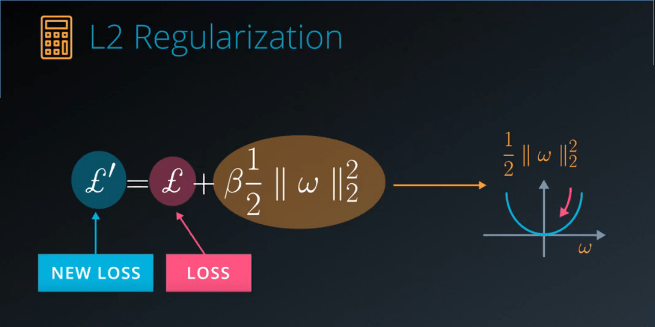
优雅一点的方法是,在 loss function 中,添加一个 weights 的和的二次方. 如果 weights 过大,loss 则会变得很大,从而在一定程度上限制 weights 的范围。这个方法只需要调整 loss function,不需要改变网络的结构。
最近比较流行的方法是 dropout. Dropout 会在训练的时候,随机地强行关闭一部分Activation,使得它们无论接受何种输入都不被触发。每次输入数据都随机选择被关闭的神经元,如此反复。

这样做的好处是,由于在训练时部分Activation神经元会被关闭,网络不能只依赖某个神经元来得到正确结果,逼迫网络产生冗余,使之变得robust,不容易出现 overfitting.


在训练时,dropout会随机关闭部分Activation(例如1/2)。在预测时,dropout则不应该关闭Activation。因此,为了让训练时和预测时的scale一致,在训练时应该将Activation的输出结果放大(比如2倍),用来弥补被关闭的神经元的输出。

CNN – Convolutional Neural Networks
将深度学习应用到图片识别是可行的。Convolutional Neural Network (CNN) 非常适合干这活儿。
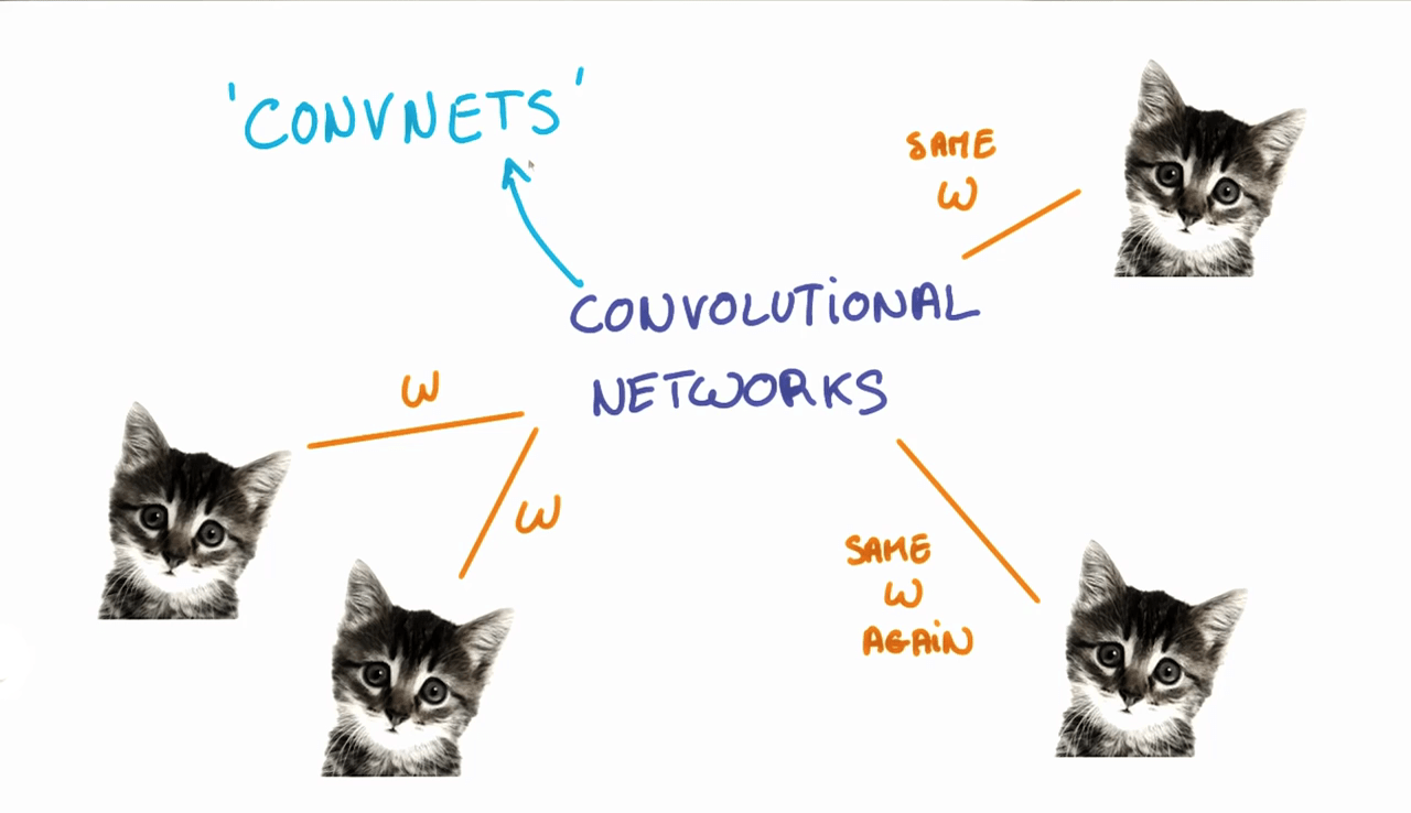
识别图片首先会遇到“位置”问题。比如,一张图片中,无论猫出现在左上角还是右下角,输入到网络中,得到的结果都应该是“这是猫”。把图片像素信息当作矩阵输入到 F=Wx+b 的网络中,不太可行。
Convolution 可以解决这个问题。
Convolution
在 CNN 中,我们可以训练一个 Filter, 让这个 Filter 从左往右,从上往下,扫描图像的每一处。如果符合这个 filter 的特征,则触发输出。这样的 Filter,称为 patch 或者 kernel.
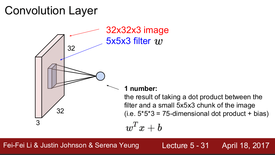
需要留意的是,我们搞了大半天,其实是为了训练 patch/kernel 里面的 parameters,为的是让这些 patches 能各自识别图像中的某些特征。比如,训练出一个 patch 能识别一只猫,那么无论这只猫在图像的左上角还是右下角,这个 patch 总会刷到这个地方,在刷到这个地方的时候即可触发输出。
还有一个叫 stride 的参数,控制这个 Patch 怎么刷。例如,strade=2, 那么它会从左往右,每次移动2个像素,换行的时候,也会往下2个像素。不同的 stride 也会得到不同的输出大小。

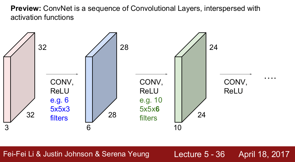
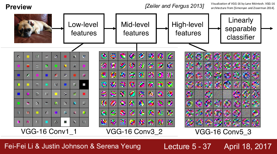
一个训练好的网络,通常会是这样的:浅层的 patches 能识别出简单的形状,比如点和线段;越深处的 patches 能基于前面的输入,识别出更复杂的图案。
Pooling
通常,在 Convolution Layer 之后,会加入 Pooling Layer。 Pooling Layer 会进行 Downsampling, 保留重要信息,减少输入到下一层的数据量。
常用的是 Max Pooling,它把最能够触发到下一层的数据保留,去除其他数据。


LeNet

后面用到的模型是基于LeNet的。 这个作业中,使用的最终模型如下:
– 前面是2个(Convolution + Activation + Pooling)的组合。Convolution 层使用了 5×5 filter, 1×1 stride. Pooling 使用 2×2 kernel, 2×2 stride.
– 后面接着3个 Fully Connected Layers,每个 FC 包含 Linear + Activation. Layer 3 从 input=400 features 得到 output=120 features, Layer 4 从 input=120 得到 output=84. 最后一层 layer 5 从 input=84 得到 43 个 logits (这个交通标识数据集一共有43个不同类别的标识)
代码实现
读取数据
用pickle解开训练和测试数据集(数据集从Udacity课程页面中下载,这里不提供链接)
图像数据存放到 X_train 和 X_test 中。label(预期的分类结果)存放在 y_train 和 y_test 中。
[cc lang=”python”]
# Load pickled data
import pickle
# Location where saved the training and testing data
training_file = ‘/home/feichashao/traffic-signs-data/train.p’
testing_file = ‘/home/feichashao/traffic-signs-data/test.p’
with open(training_file, mode=’rb’) as f:
train = pickle.load(f)
with open(testing_file, mode=’rb’) as f:
test = pickle.load(f)
X_train, y_train = train[‘features’], train[‘labels’]
X_test, y_test = test[‘features’], test[‘labels’]
[/cc]
检查数据集大小。
[cc lang=”python”]
import numpy as np
# Number of training examples
n_train = len(X_train)
# Number of testing examples.
n_test = len(X_test)
# What’s the shape of an traffic sign image?
image_shape = X_train[0].shape
# How many unique classes/labels there are in the dataset.
n_classes = len(np.unique(y_train))
print(“Number of training examples =”, n_train)
print(“Number of testing examples =”, n_test)
print(“Image data shape =”, image_shape)
print(“Number of classes =”, n_classes)
[/cc]
[cc lang=”text”]
Number of training examples = 39209
Number of testing examples = 12630
Image data shape = (32, 32, 3)
Number of classes = 43
[/cc]
随机检查一张图片。
[cc lang=”python”]
### Data exploration visualization goes here.
import random
import numpy as np
import matplotlib.pyplot as plt
%matplotlib inline
index = random.randint(0, len(X_train))
image = X_train[index].squeeze()
plt.figure(figsize=(1,1))
plt.imshow(image)
print(y_train[index])
[/cc]
38 – Keep right (靠右行驶)

嗯,图片太暗,要认真看才能看清。在后面,要先对图像进行预处理,再进行训练。
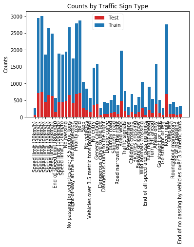
画出各种类型交通标识的数量分布。这里的分布不算平均。按照感觉,分布越平均约有利于提高实际测试时的准确度。如果分布偏向于某一类别,进行预测的时候它可能会瞎猜分布最高的类别。(就像我们考试喜欢选C)
[cc lang=”python”]
### Plot the number of each traffic sign.
import csv
test_label_counts = np.zeros(n_classes)
train_label_counts = np.zeros(n_classes)
sign_name_list = []
with open(‘signnames.csv’) as csvfile:
reader = csv.DictReader(csvfile)
for row in reader:
sign_name_list.append(row[‘SignName’])
#print(sign_name_list)
for label in y_test:
test_label_counts[label] += 1
for label in y_train:
train_label_counts[label] += 1
plt.xticks(rotation=90)
ind = np.arange(n_classes)
p1 = plt.bar(ind, test_label_counts, width=0.8, color=’#d62728′)
p2 = plt.bar(ind, train_label_counts, width=0.8, bottom=test_label_counts)
# plt.rcParams[‘figure.figsize’] = (20.0, 40.0)
plt.ylabel(‘Counts’)
plt.xticks(ind, sign_name_list)
plt.title(‘Counts by Traffic Sign Type’)
plt.legend((p1[0], p2[0]), (‘Test’, ‘Train’))
plt.show()
[/cc]
数据预处理
首先是打乱顺序。如果不打乱顺序,那么在训练时,神经网络可能会连续看到几百次同一个标识(比如”stop”),影响训练效果。如果考试题连续100题标准答案都是A,学生以后可能会蒙着眼选A。
[cc lang=”python”]
from sklearn.utils import shuffle
X_train, y_train = shuffle(X_train, y_train)
[/cc]
将彩色图片转换为灰度图片,减少特征(features)数量。对交通标志而言,灰度图的辨识度不比彩色图差太多。(”stop”之类的标识有明显的红色,不过在灰度图中也能辨认出是”stop”)。
然后进行 CLAHE (Contrast-limited adaptive histogram equalization)变换。CLAHE 是直方图均衡的一种算法,有助于提升图像对比度。
[cc lang=”python”]
# Convert images into grayscale and perform CLAHE to normalize image.
# Reference:
# http://docs.opencv.org/3.1.0/d5/daf/tutorial_py_histogram_equalization.html
# http://docs.opencv.org/3.2.0/d7/d1b/group__imgproc__misc.html
import cv2
def clahe_cvt(original_images, clahe_images):
clahe = cv2.createCLAHE()
for i in range(len(original_images)):
image = original_images[i].squeeze()
gray_image = cv2.cvtColor(image, cv2.COLOR_RGB2GRAY)
clahe_images[i,:,:,0] = clahe.apply(gray_image)
X_train_cl = np.ndarray(shape=(n_train, image_shape[0], image_shape[1], 1), dtype=np.uint8)
X_test_cl = np.ndarray(shape=(n_test, image_shape[0], image_shape[1], 1), dtype=np.uint8)
clahe_cvt(X_train, X_train_cl)
clahe_cvt(X_test, X_test_cl)
[/cc]
选一张图进行对预处理操作进行校验。可以看到,这个”stop”的灰度图没有走样,人类可以辨认。
[cc lang=”python”]
# Pick some pictures to verify the above pipeline works well.
index = random.randint(0, len(X_test_cl))
image = X_test_cl[index].squeeze()
plt.figure(figsize=(1,1))
plt.imshow(image, ‘gray’)
print(sign_name_list[y_test[index]])
[/cc]

最后,将输入图像的数值范围从 0~255 调整为 -128~127,使均值为0(zero-center).
[cc lang=”python”]
### Normalize data
### Convert input from range 0 ~ 255 to -128 ~ 127
X_train_cl = X_train_cl.astype(int)
X_test_cl = X_test_cl.astype(int)
X_train_cl -= 128
X_test_cl -= 128
print(X_train_cl.dtype)
print(np.unique(X_train_cl[2]))
[/cc]
将训练数据集分成80/20两份,20那份作为校验集(validation set),用于在训练的时候对训练效果进行校验。
[cc lang=”python”]
### Split the data into training/validation/testing sets here.
from sklearn.model_selection import train_test_split
X_train_cl, X_validation_cl, y_train, y_validation = train_test_split(X_train_cl, y_train, test_size=0.2, random_state=0)
[/cc]
TensorFlow实现LeNet
用Tensorflow把LeNet模型堆砌出来。
[cc lang=”python”]
import tensorflow as tf
from tensorflow.contrib.layers import flatten
def LeNet(x):
# Arguments used for tf.truncated_normal, randomly defines variables for the weights and biases for each layer
mu = 0
sigma = 0.1
# Layer 1: Convolutional. Input = 32x32x1. Output = 28x28x6.
conv_W1 = tf.Variable(tf.truncated_normal(shape=(5, 5, 1, 6), mean=mu, stddev=sigma))
conv_b1 = tf.Variable(tf.zeros(6))
conv1 = tf.nn.conv2d(x, conv_W1, strides = [1, 1, 1, 1], padding = ‘VALID’) + conv_b1
# Activation.
conv1 = tf.nn.relu(conv1)
# Pooling. Input = 28x28x6. Output = 14x14x6.
conv1 = tf.nn.max_pool(conv1, ksize = [1, 2, 2, 1], strides = [1, 2, 2, 1], padding = ‘VALID’)
# Layer 2: Convolutional. Output = 10x10x16.
conv_W2 = tf.Variable(tf.truncated_normal(shape=(5, 5, 6, 16), mean=mu, stddev=sigma))
conv_b2 = tf.Variable(tf.zeros(16))
conv2 = tf.nn.conv2d(conv1, conv_W2, strides = [1, 1, 1, 1], padding = ‘VALID’) + conv_b2
# Activation.
conv2 = tf.nn.relu(conv2)
# Pooling. Input = 10x10x16. Output = 5x5x16.
conv2 = tf.nn.max_pool(conv2, ksize = [1, 2, 2, 1], strides = [1, 2, 2, 1], padding = ‘VALID’)
# Flatten. Input = 5x5x16. Output = 400.
fc0 = flatten(conv2)
# Layer 3: Fully Connected. Input = 400. Output = 120.
fc1_W = tf.Variable(tf.truncated_normal(shape=(400, 120), mean=mu, stddev=sigma))
fc1_b = tf.Variable(tf.zeros(120))
fc1 = tf.matmul(fc0, fc1_W) + fc1_b
# Activation.
# fc1 = tf.nn.relu(fc1)
# Play around, append dropout.
fc1 = tf.nn.dropout(fc1, keep_prob = 0.8)
# Layer 4: Fully Connected. Input = 120. Output = 84.
fc2_W = tf.Variable(tf.truncated_normal(shape=(120, 84), mean=mu, stddev=sigma))
fc2_b = tf.Variable(tf.zeros(84))
fc2 = tf.matmul(fc1, fc2_W) + fc2_b
# Activation.
fc2 = tf.nn.relu(fc2)
# Layer 5: Fully Connected. Input = 84. Output = 43.
fc3_W = tf.Variable(tf.truncated_normal(shape=(84, 43), mean=mu, stddev=sigma))
fc3_b = tf.Variable(tf.zeros(43))
logits = tf.matmul(fc2, fc3_W) + fc3_b
return logits
[/cc]
定义输入输出和cost function.
这里使用了 AdamOptimizer 进行优化。相比于普通的 Gradient Descent, Adam 会自动动态调节 learning rate, 在训练的后期可以 fine tune,进一步降低错误率。(参考 https://stats.stackexchange.com/questions/184448/difference-between-gradientdescentoptimizer-and-adamoptimizer-tensorflow)
[cc lang=”python”]
# Set up placeholders for input
x = tf.placeholder(tf.float32, (None, 32, 32, 1))
y = tf.placeholder(tf.int32, (None))
one_hot_y = tf.one_hot(y, 43)
# Set up training pipeline
rate = 0.001
logits = LeNet(x)
cross_entropy = tf.nn.softmax_cross_entropy_with_logits(logits, one_hot_y)
loss_operation = tf.reduce_mean(cross_entropy)
optimizer = tf.train.AdamOptimizer(learning_rate = rate)
training_operation = optimizer.minimize(loss_operation)
# Evaluation
correct_prediction = tf.equal(tf.argmax(logits, 1), tf.argmax(one_hot_y, 1))
accuracy_operation = tf.reduce_mean(tf.cast(correct_prediction, tf.float32))
saver = tf.train.Saver()
def evaluate(X_data, y_data):
num_examples = len(X_data)
total_accuracy = 0
sess = tf.get_default_session()
for offset in range(0, num_examples, BATCH_SIZE):
batch_x, batch_y = X_data[offset:offset+BATCH_SIZE], y_data[offset:offset+BATCH_SIZE]
accuracy = sess.run(accuracy_operation, feed_dict={x: batch_x, y: batch_y})
total_accuracy += (accuracy * len(batch_x))
return total_accuracy / num_examples
[/cc]
设置epochs和batch_size, 开启 tensorflow session 进行训练。
TensorFlow训练LeNet
[cc lang=”python”]
# Training
EPOCHS = 15
BATCH_SIZE = 128
with tf.Session() as sess:
sess.run(tf.global_variables_initializer())
num_examples = len(X_train_cl)
print(“Training…”)
print()
for i in range(EPOCHS):
X_train_cl, y_train = shuffle(X_train_cl, y_train)
for offset in range(0, num_examples, BATCH_SIZE):
end = offset + BATCH_SIZE
batch_x, batch_y = X_train_cl[offset:end], y_train[offset:end]
sess.run(training_operation, feed_dict={x: batch_x, y: batch_y})
validation_accuracy = evaluate(X_validation_cl, y_validation)
print(“EPOCH {} …”.format(i+1))
print(“Validation Accuracy = {:.3f}”.format(validation_accuracy))
print()
saver.save(sess, ‘lenet-normal-1’)
print(“Model saved”)
[/cc]
[cc lang=”text”]
Training…
EPOCH 1 …
Validation Accuracy = 0.234
EPOCH 2 …
Validation Accuracy = 0.601
EPOCH 3 …
Validation Accuracy = 0.767
EPOCH 4 …
Validation Accuracy = 0.838
EPOCH 5 …
Validation Accuracy = 0.881
EPOCH 6 …
Validation Accuracy = 0.905
EPOCH 7 …
Validation Accuracy = 0.923
EPOCH 8 …
Validation Accuracy = 0.923
EPOCH 9 …
Validation Accuracy = 0.940
EPOCH 10 …
Validation Accuracy = 0.937
EPOCH 11 …
Validation Accuracy = 0.949
EPOCH 12 …
Validation Accuracy = 0.946
EPOCH 13 …
Validation Accuracy = 0.956
EPOCH 14 …
Validation Accuracy = 0.948
EPOCH 15 …
Validation Accuracy = 0.958
Model saved
[/cc]
[cc lang=”python”]
# Test the model against test set
with tf.Session() as sess:
saver.restore(sess, tf.train.latest_checkpoint(‘.’))
test_accuracy = evaluate(X_test_cl, y_test)
print(“Test Accuracy = {:.3f}”.format(test_accuracy))
[/cc]
[cc lang=”text”]
Test Accuracy = 0.914
[/cc]
调整参数
// TODO make a plot?
Tried decreasing the learning rate to 0.0005/0.0008. Use the default learning rate 0.001, the accuracy can reach 0.965, but after tunning, the accuracy dropped to around 0.940. Lower the learning rate can help avoiding overfitting, but in this case it is not necessary.
Tried adding a dropout (keep_prob=0.5) to layer 3 (the first fc layer), but the accuracy dropped to 0.830. Then tried remove the relu of layer 3, and add a dropout (keep_prob=0.8), the accuracy became 0.951. Though it is not as high as the default LeNet, but I keep it as it would be more robust.
实际路牌识别效果
在百度地图街景中,截取了G8高速北京段的几个交通标识。看看上面训练出来的网络,能不能识别出来祖国的交通标识。
[cc lang=”python”]
# preprocess: $ for i in {1..13}; do convert $i.png -resize 32×32\! test$i.png; done
from scipy import misc
path = ‘/home/feichashao/traffic-signs-data/’
def read_image(filename):
image = misc.imread( path + filename)
return image
image_files = [‘test1.png’, ‘test5.png’, ‘test7.png’, ‘test10.png’, ‘test11.png’]
new_labels = np.array([38, 8, 7, 0, 17], np.int)
new_images = [read_image(filename) for filename in image_files]
[/cc]
[cc lang=”python”]
### Sign 0 – label 38 – Keep Right
plt.figure(figsize=(1,1))
plt.imshow(new_images[0])
print(new_images[0].shape)
[/cc]

[cc lang=”python”]
### Sign 1 – label 8 – Limit 120 km/h
plt.figure(figsize=(1,1))
plt.imshow(new_images[1])
print(new_images[1].shape)
[/cc]

[cc lang=”python”]
### Sign 2 – label 7 – Limit 100 km/h
plt.figure(figsize=(1,1))
plt.imshow(new_images[2])
print(new_images[2].shape)
[/cc]

[cc lang=”python”]
### Sign 3 – label 0 – Limit 20 km/h
plt.figure(figsize=(1,1))
plt.imshow(new_images[3])
print(new_images[3].shape)
[/cc]

[cc lang=”python”]
### Sign 4 – label 17 – No entry
plt.figure(figsize=(1,1))
plt.imshow(new_images[4])
print(new_images[4].shape)
[/cc]

对以上测试图像进行预处理。(预处理过程跟之前的一致)
[cc lang=”python”]
### Preprocess.
print(new_images[0].dtype)
clahe = cv2.createCLAHE()
tmp = np.ndarray(shape=(len(new_images), 32, 32, 1), dtype=np.int)
for i in range(len(new_images)):
image = new_images[i].squeeze()
gray_image = np.ndarray(shape=(32,32,1), dtype=np.uint8)
#gray_image[:,:,0] = cv2.cvtColor(image, cv2.COLOR_RGB2GRAY)
gray_image[:,:,0] = cv2.cvtColor(image, cv2.COLOR_RGB2GRAY)
cl_image = clahe.apply(gray_image)
cl_image = cl_image.astype(int)
cl_image -= 128
tmp[i,:,:,0] = cl_image
new_images = tmp
[/cc]
[cc lang=”python”]
with tf.Session() as sess:
saver.restore(sess, tf.train.latest_checkpoint(‘.’))
new_softmax = tf.nn.softmax(logits)
topk = tf.nn.top_k(new_softmax, k = 5)
topk_val , indexes = sess.run(topk, feed_dict={x: new_images})
[/cc]
32×32的图像输入到网络后,会得到 43 个 logit 的输出。网络会取得分最高的 logit,作为最终答案。
可以通过可视化的方式,查看每个图像对应的 logit 值。
[cc lang=”python”]
### Visualize top 5 softmax.
def visualize_top5(indexes, probs):
plt.rcdefaults()
fig, ax = plt.subplots()
y_pos = np.arange(len(indexes))
ax.barh(y_pos, probs)
ax.set_yticks(y_pos)
ax.set_yticklabels([sign_name_list[i] for i in indexes])
ax.invert_yaxis()
ax.set_xlabel(‘Softmax’)
ax.set_title(‘Softmax on Top 5 indexes’)
[/cc]
[cc lang=”python”]
visualize_top5(indexes[0], topk_val[0])
“””
Classified as 38 (Keep right) correctly.
“””
[/cc]

[cc lang=”python”]
visualize_top5(indexes[1], topk_val[1])
“””
label 8 – Limit 120 km/h
Should be label 8 (120km/h), but classified as label 0 (limit 20km/h)
“””
[/cc]

[cc lang=”python”]
visualize_top5(indexes[2], topk_val[2])
“””
label 7 – Limit 100 km/h
Should be label 7 (limit 100km/h), but classified as stop.
“””
[/cc]

[cc lang=”python”]
visualize_top5(indexes[3], topk_val[3])
“””
label 0 – Limit 20 km/h
should be label 0 (limit 20km/h), but classified as Road narrows on the right.
“””
[/cc]

[cc lang=”python”]
visualize_top5(indexes[4], topk_val[4])
“””
label 17 – No entry
Correct.
“””
[/cc]

从上面结果可以看到,“靠右行驶”(keep right)和“不准进入”(no entry)两个标识被正确识别了。而其余3个限速标识都识别出错。
可能的原因是,“靠右行驶”和“不准进入”特征明显,而限速标识还涉及到多个数字,容易混淆。